Generalizing Long Run Performance Beyond Finite MCs

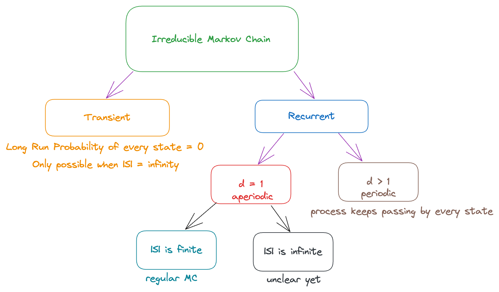
Recall this from the previous page:

Note that we’re only talking about irreducible MCs for now. We already know what happens in all the cases except when we have a recurrent aperiodic MC with infinite states.

We will now try to generalize the results we’ve obtained for a regular MC to a recurrent aperiodic MC with infinite states. That is, we want to answer the question: when there are infinite states, how do we derive the regularity?

Is it possible that we have $P(\text{return}) = 1$ and $E[\text{Return Time}] = \infty$? Then it still seems “impossible” to return (even though the probability is $1$). We want to be able to intrepret this corectly (and gain intuition about this).

Generalising Main Theorem

Consider a recurrent MC.

definition

First Return Time: $R_i = \min\{n \geq 1, X_n =i\}$

In words, it is the first time that the process $X_n$ returns to $i$.

Recall that we defined $f_{ii}^{(n)}$ (first return probability) to be “starting with $i$, what is the probability that the first return to $i$ happens at $n$th step).

So, what is the relationship between $R_i$ and $f_{ii}^{(n)}$?

Clearly, we can express it as: $f_{Ii}^{(n)} = P(R_i = n|X_0=i)$

In other words, we can say that $f_{ii}^{(n)}$ is the “probability mass” of $R_i$ at $n$, i.e., $f_{ii}^{(n)}$ gives us the probability that $R_i=n$.

For recurrent states, we know that $f_{ii}=1$, i.e., $\sum_{n} f_{ii}^{(n)} = 1$. Therefore, we can calculate $E[R_i|X_0=i]$, which can be interpreted as the average first return time or (more commonly known as) the mean duration between visits.

By definition of “mean” (expectation), we can write it as such:

$$m_i =E[R_i |X_0=i] = \sum_{n=1}^\infty nP(R_i=n|X_0=i) = \sum_{n=1}^\infty nf_{ii}^{(n)}$$

Note that we can only define $m_i$ when $f_{ii} = 1$. When we have $f_{ii} < 1$, then the probability that there are infinitely many steps between 2 visits is non-zero, and equal to $1-f_{ii}$ so the expectation will be infinity (which is not very meaningful).

Limit Theorem

definition

For any recurrent irreducible MC, define:

$$m_i = E[R_i|X_0=i] = \sum_{n=1}^\infty nf_{ii}^{(n)}$$

Then,

1. For any $i, j \in S$,

   $$\lim_{n \to \infty} \sum_{k=1}^n P_{ij}^{(k)}/n = 1/m_j$$

2. If $d=1$, then

   $$\lim_{n \to \infty} P_{ij}^{(n)} = 1/m_j$$

3. If $d > 1$, then

   $$\lim_{n \to \infty} P_{jj}^{(nd)} = d/m_j$$

Note that the theorem applies for MCs with infinitely many states too! It also applies for periodic MCs.

Interpretation

Let’s try to interpret the theorem:

1. Consider a fixed $j$ and observe that for all $i$, the “average transition probability” (in the long-run) is the same, and equal to $1/m_j$. This seems intuitive because we can think of a transition to $j$ as a “success” and a transition to any other state as a “failure” and model it as a geometric distribution. Then, we know that if the probability of success is $p$, the mean time for success is $1/p$. In this case, transitioning to any other state preserves the probability of success (i.e., it does not change $p$ because every state has the same probability of transition to $p$) and so, it does indeed fit well as a geometric distribution. For an aperiodic MC, in the long-run, the probability of transitioning from $i \to j$ converges to $1/m_j$.

   Note that this theorem applies to periodic MCs as well, but the analogy of a geometric distribution only holds for an aperiodic MC.

2. In the first part of the theorem, we’re considering the limit of the average transition probability from $i \to j$. But when the MC is aperiodic, we’re saying that the $n$-th step probability $P_{ij}^{(n)}$ itself (not the average) converges to a fixed value, equal to $1/m_j$.

   This looks very similar to the regular MC case - we know that in the long-run, $P_{ij}^{(n)} = \pi_j$ when we have finitely many states (recall that for a regular MC with finite states, $P^{(n)}$ converges to a “fixed” matrix where every row is equal to the limiting distribution). This should give a hint that $\pi_j = 1/m_j$ 😲

   Note that the average of a convergent series is determined by the “long-run terms” and since there are infinitely many terms which are equal to the limit (they dominate the initial few terms which may be different from the limit), the average is also equal to the limit. This is how we can understand that (2) and (1) are compatible/consistent with each other.

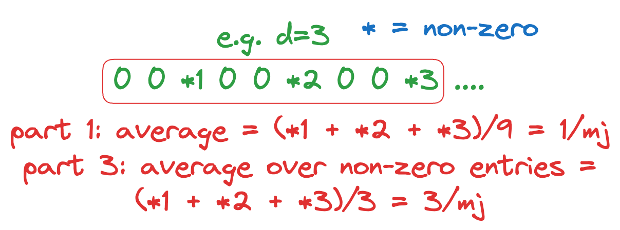
3. In the third part, notice that we’re only considering the probability of returning to $j$ when we start from $j$ itself. If we start from any other state, we can’t make any claims since we don’t know how many steps it takes to reach $j$. For any $k$ that is NOT a multiple of the period $d$, obviously $P_{jj}^{(k)} = 0$. So, we only consider the limit of the non-zero entries, i.e., entries of $P^{(k)}$ where $k$ is a multiple of $d$. In this case, we claim that the limit exists, and is equal to $d/m_j$.

   It is natural to expect $d$ to appear on the RHS because if we look at the first result, the “average” is brought down (by a factor of $d$) by all the $d-1$ zero-entries between every 2 multiples of $d$. But in this case, we’re removing all these zero-entries and only considering multiples of $d$, and so we expect the “average over non-zero entries” to be $d$ times higher.

   

   Basically, we expect the non-zero entries, $P_{jj}^{(nd)}$ to converge to $d/m_j$ as $n \to \infty$.

   Until now, we didn’t know what would happen for a periodic MC in the long run, since it doesn’t converge. While that is still true, we’ve shown that the subsequence formed by the non-zero entries does indeed converge (and so, we can make more sense out of the process).

Remarks

The mean duration between visits, $m_i$, can be finite or infinite:

• Infinite: When $m_j = \infty$, the limiting probability at each state is $0$, although it is recurrent. We call such a MC to be null recurrent. For example, consider the symmetric random walk with $p=1/2$ and no absorbing state. Note that it is still recurrent (there’s only one class so it must be recurrent).
• Finite: When $m_j < \infty$, the limiting probability at each state is $1/m_j$. In such a case, we call it a positive recurrent MC. e.g. Random walk with $p < 1/2$ (process eventually reaches 0) and “reflection” at $0$, i.e., $P(X_n=1|X_{n-1}=0) = 1$ When $d > 1$, we can only consider the steps $n$d. When $d=1$, the limiting probability is positive, which means that it is a regular MC.

info

The notion of “null recurrence” only applies to MCs with $\infty$ states. For a MC with finite states, a state can never be null-recurrent.

Basic Limit Theorem

We can generalize the results from the previous theorem by only considering those MCs that have $m_j < \infty$. This gives us the Basic Limit Theorem.

theorem

Basic Limit Theorem

For a positive recurrent ($m_j < \infty$), irreducible, and aperiodic MC,

• $\lim_{n \to \infty} P_{ij}^{(n)}$ exists for any $i,j$ and is given by:
  $$\lim_{n \to \infty} P_{ij}^{(n)} = \lim_{n \to \infty} P_{jj}^{(n)} = \frac 1 {m_j}$$
• If $\pi$ is the solution to the equation $\pi P = \pi$, then we have:
  $$\pi_j = \frac 1 {m_j}$$

Note:

• A positive recurrent, irreducible, aperiodic MC is called an ergodic MC. Hence, the basic limit theorem applies to all ergodic MCs.
• All regular MCs are also ergodic MCs. Why? Because if there are finite states (and it is irreducible so all of them must be recurrent), the limiting probability on each state is non-zero, hence it is positive recurrent.
• We do NOT require the MC to have finite/infinite states for the theorem to hold.

In general, it’s quite difficult to prove the “positive recurrent” property of a MC with inifinite states, so we normally deal with MCs with finite states (for which we can apply the theorem from the previous page for regular MCs)

How do we calculate $m_j$? Using the second part of the theorem, we can first solve $\pi = \pi P$ to find the limiting distribution, and then take its reciprocal to obtain all the $m_j$’s. This gives us another interpretation for $\pi_j$ ⇒ knowing $\pi_j$ (and hence, $1/\pi_j$) also tells us the mean duration between visits.

Sometimes, it’s easier to find $m_i$ rather than $\pi_i$ (generally when we have infinite states). Exampe: A MC representing the number of consecutive successes of an binomial trials (with probability of success = $p$). To calculate $m_i$ in such a case, we need to find $f_{ii}^{(n)}$ for all values of $n$ and then use the definition of $m_i = \sum_{n=1}^\infty nf_{ii}^{(n)}$.

Reducible Chains

Until now, we’ve been talking only about irreducible chains (and all the theorems only apply to irreducible chains). So, what do we do for reducible chains?

Intuitively we know that we can “reduce” (i.e., decompose) the reducible chain into irreducible sub-chains (each subchain consists of states in the same communication class).

Then, in the long-run, the limiting probability of the transient classes is zero. Moreover, we can find the probability of entering any recurrent class using FSA (by treating every recurrent class as an absorbing state since the process can never leave the recurrent class, i.e., no outoing arrows from the recurrent class).

Then, within each recurrent class of the reducible MC, we can check the period $d$.

• If $d > 1$, then the limit of the subsequence is $d/m_j$ for every state $j$ in the class (only true if the process starts at state $j$).
• If $d=1$
  • If the class has finite states, then we can find out the limiting probability (since it is a regular markov “subchain”) using $\pi = \pi P$
  • If the class has $\infty$ states, then the limiting probability at each state is either zero (if it is null recurrent) or can be obtained by $\pi = \pi P$ if it is positive recurrent.

Now we know what happens whenever we have a recurrent class. Next, we’ll try to incorporate these results into a general MC so that we can understand the long-run probability of every state (note: not every class).

Long-Run Performance in General Markov Chains

As a quick recap, currently we know how to:

• Find the probability of a process entering any recurrent class (using FSA)
• Find the limiting probability of each state within the recurrent class (using $\pi = \pi P$) if the period $d=1$. (of course, if $d \neq 1$, then there is no limiting distribution since the limit does not converge)

If we can combine both, we can get the results for a general markov chain. Basically, we’re trying to find $P^{(n)}$ as $n \to \infty$ for a general MC now (for a regular MC, we already know that $P^{(n)}$ will consist of all rows equal to $\pi$ but we don’t expect this to be the case for a general MC).

Intuitively (using conditional probability), we know that the limiting probabiilty (if it exists) at a state $j$ is equal to the probability of entering $j$’s recurrent class times the limiting probability $\pi_j$ in its own class.

Formally, consider $j \in C_k$ where $C_k$ is a recurrent class. Then, we can set up a new MC and find the entering probability:

$$u_{k|\pi_0} = P(\text{entering } C_k|X_0 \sim \pi_0)$$

Once the process enters $C_k$, it never leaves. Hence, we can restrict the process (i.e., consider the sub-chain) on $C_k$ only. Clearly, the new MC restricted on $C_k$ is irreducible and recurrent (since it is formed by states in the same class).

Then, we can find $m_j$ for state $j$ by solving $\pi = \pi P$.

Hence, if we repeat generating $X_0$ and making $n$ jumps for sufficiently large $n$ (i.e., $n \to \infty$), then:

$$\pi_j = P(\text{entering } C_k | X_0 \sim \pi_0) \times P(\text{staying at }j | \text{entered } C_k) \\ = u_{k|\pi_0} \pi_{j|k} = u_{k|\pi_0}/m_j$$

Procedure

For the sake of clarity and completeness, we outline the entire procedure to analyze the long-run performance of ANY general MC.

1. Find all the classes $C_k$

2. Set up a new MC where every recurrent class is denoted by one state. Then, find $P(\text{absorbed in recurrent class } C_k | X_0= i)$ denoted by $u_{k|i}$ → this gives the probability of entering any recurrent class, given the initial distribution.

3. We can ignore all transient classes 😲 because the process will eventually leave them in the long-run, i.e., their long-term probability is zero.

4. For every recurrent class $C_k$, we find the period $d$.

   1. Aperiodic (d=$1): find the corresponding limiting distribution of state $j in this class, denoted by $\pi_{j|k}$, by considering the sub-MC restricted on $C_k$
   2. Periodic ($d > 1$): there is NO limiting distribution, but we can still check the long-run proportion of time in each state by finding $m_j$ (i.e., we can still find $\pi$ but the interpretation is different in this case)

5. Consider the initial state $X_0 = i$

   1. If $j$ is transient, then $\pi_j =0$

   2. If $j \in C_k$ is recurrent, then:

      $$\pi_{j|i} = u_{k|i}\pi_{j|k}$$

6. Finally, given the initial distribution $X_0 \sim \pi_0$, then:

   $$\pi_{j|\pi_0} = \sum_{i \in S} \pi_{j|i} \pi_0(i)$$